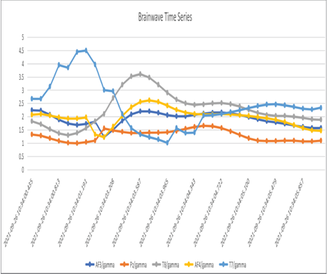
The streaming of data from an IoT device, like a BCI, is an ideal fit for time series analysis. The data in this context is ideal because the data includes a timestamp and is received in order, both of which are time series data characteristics. Figure 7.29 shows a time series line chart that represents a chronological series of brain wave readings that were ingested.

FIGURE 7.29 A brain wave time series chart
The more data you consume and store, the greater your ability to discover trends and spot anomalies. This kind of data is also very useful for predictive analysis. In Chapter 5, “Transform, Manage, and Prepare Data,” you used this data to discover the median ranges of frequencies of brain wave readings per frequency. You then used those values in Exercise 7.5 to predict which brainjammer brain wave scenario is taking place in real time.
Another characteristic when working with time series data is the storage folder structures based on date and time, as follows:
{Region}/{SubjectMatter}/out/{yyyy}/{mm}/{dd}/{hh}/
EMEA/brainjammer/in/2022/08/17/17
You have seen this pattern in many places in this book. Structuring your data in this manner helps PolyBase and DataFrame queries perform better. They perform better because the amount of data in each directory would be smaller when compared to storing data for an entire day or week in a single file. Finding an optimal partition for your data is very important if you want a healthy, non‐latent data solution. It is possible to take this naming convention to the file level, as follows:
filename_YYYY_MM_DD_HH_mm.parquet
brainwaves_2022_08_17_17_22.parquet
This means the queries can be optimized to run on data files down to the minute time frame, which might be the optimal design for a data analytics solution. If the ingestion frequency is once per minute, then you have attained equilibrium with the law of 60 once again.
Design and Create Windowed Aggregates
When you think about streaming aggregate functions, the functions in Table 3.20 should come to mind, for example, AVG, COUNT, MAX, and MIN. When you use the PERCENTILE_CONT and PERCENTILE_DISC aggregate functions in the streaming context, you restrict the execution of those aggregates to a set of data in a prescribed time frame, for example, running the AVG function on all received data within the last 5 seconds. The configuration of that time window is achieved using temporal windows, which you read about in this chapter and learned in detail in Chapter 3. Again, the types of temporal windowing functions are tumbling, hopping, sliding, session, and snapshot. Take this one step further, you can aggregate the temporal windowing functions themselves. The following syntax illustrates how to aggregate a windowed function:
SELECT
System.Window().Id AS WindowId,
System.TimeStamp() AS IngestionTime,
PERCENTILE_CONT(0.5) OVER (ORDER BY brainwaves.ALPHA) AS medianAPLHA,
PERCENTILE_CONT(0.5) OVER (ORDER BY brainwaves.BETA_H) AS medianBETA_H,
PERCENTILE_CONT(0.5) OVER (ORDER BY brainwaves.BETA_L) AS medianBETA_L,
PERCENTILE_CONT(0.5) OVER (ORDER BY brainwaves.GAMMA) AS medianGAMMA,
PERCENTILE_CONT(0.5) OVER (ORDER BY brainwaves.THETA) AS medianTHETA
FROM brainwaves
GROUP BY WindowId, IngestionTime,
Windows(
Window(’10s Tumble’, TumblingWindow(second, 10)),
Window(’10s Hop’, HoppingWindow(second, 10, 5)),
Window(’30s Session’, SessionWindow(second, 30, 60)),
Window(’30s Sliding’, SlidingWindow(second, 30)))
The Windows() function provides the technology to implement windowed aggregates. As you can see, the Windows() function accepts parameters of multiple window definitions, like tumbling, hopping, session, and sliding. The window Id is the first parameter of the Window() function and is referenced in the SELECT statement using the following code snippet:
System.Window().Id
To learn more about implementing windowed aggregates, complete Exercise 7.7. Note that you must have completed Exercise 7.3 in order to successfully complete this exercise, as it includes some resources you need to update.


