
- Log in to the Azure portal at https://portal.azure.com➢ navigate to the Azure Synapse Analytics workspace you created in Exercise 3.3➢ select the Manage hub ➢ start the SQL pool (the same one you used in Exercise 7.3) ➢ select the Data hub ➢and then create a new table named BrainwaveWindowMedians. The syntax is in the BrainwaveWindowMedians.sql file in the Chapter07/Ch07Ex07 directory on GitHub.
- Navigate to the Azure Stream Analytics job you created in Exercise 3.17➢ select Outputs from the navigation menu ➢ select the synapse alias you created in Exercise 7.3➢ change the value in Table to the following ➢ and then click Save.
brainwaves.BrainwaveWindowMedians - Select Query from the navigation menu ➢ add the query in the file StreamAnalyticsQuery.txt, which is located in the Chapter07/Ch07Ex07 directory on GitHub ➢ click the Save Query button ➢ and then start the Azure Stream Analytics job.
- Download, uncompress, and use the brainjammer.exe located in the brainjammer.zip file in the Chapter07/Ch07Ex03 directory on GitHub ➢ perform the same action as performed in step 6 of Exercise 7.3 (see Figure 7.13).
- Once the brain wave streaming is complete, navigate to the Azure Synapse Analytics workspace you created in Exercise 3.3 and view the newly added rows on the [brainwaves].[BrainwaveWindowMedians] table. Use the following query, for example:
SELECT medianAPLHA, medianBETA_H, medianBETA_L, medianGAMMA, medianTHETA
FROM [brainwaves].[BrainwaveWindowMedians]
WHERE WindowId = ’10s Tumble’
ORDER BY IngestionTime
- Stop the Azure Stream Analytics job, and then stop the Azure Synapse Analytics SQL pool.
The first action in Exercise 7.7 was to create a new table to store the stream of brain wave data readings. In addition to the frequency columns, there are columns named WindowId and IngestionTime. When you implement windowed aggregates, each window is allocated an identifier. They can be any string value, such as “20 Seconds,” “20S,” or “twenty.” A valid WindowId should be one that is helpful toward identifying the type of aggregated window. The value stored in the IngestionTime column is the output of the System.TimeStamp() method. The method returns the date and time the brain wave reading was enqueued into Event Hubs. (There is more on this in the “Configure Checkpoints/Watermarking During Processing” section.)
Next, you updated the synapse output alias so that the result of the Azure Stream Analytics query would write the data into the table you just created. The first portion of the query should be quite familiar to you now.
The statement is contained within a WITH clause so that the desired portions of the output can be referenced from a later SELECT statement. The only difference from the previous versions of this query is the addition of the two new columns just discussed. The next portion of the query is where the windowed aggregation is implemented. It performs a GROUP BY command that begins with the new columns, followed by the Window() method. The method takes an n number of Window() methods that contain parameters WindowId and the type of and configuration of each temporal window.
The query contains four different types of windowing functions, which is interesting because you might be able to use this technique to find the one that works best. One example is in the real‐time brain wave scenario detection program, although there were many results from the tumbling window function that did not result in a match to the scenario being streamed. In addition to performing more EDA, you might consider changing the window function types and their durations to see if any result in higher matching. The approach of using many different types at the same time can help expedite the exploratory data analysis process. In this example the tumbling window will store the incoming brain wave readings for 10 seconds and then run the SELECT statement captured on that collected data. The hopping window will also store the incoming data for 10 seconds before executing the SELECT statement; however, there will be a 5‐second overlap in those 10 seconds. Refer to Figure 3.80 as a reminder of how this looks in practice. The session window captures incoming brain wave readings for at least 30 seconds and a maximum duration of 60 seconds before executing the SELECT statement. Finally, the sliding window that is commonly used with the HAVING statement will execute the SELECT statements on windows of every 30 seconds that match the HAVING pattern, something like the following:
HAVING COUNT(*)> 10
Once the streaming is complete, you can view the query results in the SQL pool. A sample query was provided and results in the output are shown in Figure 7.30.
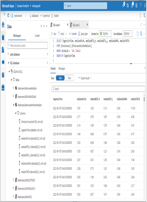
FIGURE 7.30 Windowed aggregates output
The output of the query represents the tumbling window results, which are calculated and output into the SQL pool table every 10 seconds. You could then conceivably use the scenario frequency ranges from Table 5.2 on each WindowId and determine which configuration results in the greatest match.